County-Level Analysis

Analyze GLOBE and environmental data for your county in Florida.

Write the name of your county in the quotes below. For example, county = "Broward County" or county = "Miami-Dade County" For the rest of this code notebook, we will be looking at Broward County.

county_name = "Your County Name"

# For example:
# county_name = "Broward County"

import geopandas as gpd
import pandas as pd
pd.set_option("display.max_columns", None)
import matplotlib.pyplot as plt
from matplotlib.colors import to_rgb
import seaborn as sns

First, load 1) the GLOBE Mosquito Habitat Mapper data, and 2) a file with the Florida county boundaries from the U.S. Census, which will be used to filter the data to each county.

data = gpd.read_file('https://github.com/geo-di-lab/emerge-lessons/raw/refs/heads/main/docs/data/globe_mosquito.zip')
fl = gpd.read_file('https://github.com/geo-di-lab/emerge-lessons/raw/refs/heads/main/docs/data/florida_counties.geojson')

Then, get the geographic boundaries of your county.

county = fl.loc[fl['NAMELSAD'] == county_name]

Now, we use those boundaries to filter for all GLOBE Mosquito Habitat Mapper points within your county, from 2018 to 2024.

data_county = data.sjoin(county, how="inner", predicate="within")

num_total = len(data_county)

print(f"There were {num_total} GLOBE Mosquito Habitat Mapper points recorded within {county_name} from 2018 to 2024 by community scientists.")

num_eliminated = len(data_county[data_county['BreedingGroundEliminated'] == 'true'])
print(f"Of those points, {num_eliminated} ({round(num_eliminated * 100 / num_total)}%) mosquito habitats were successfully mitigated by the community scientists, which reduces the risk for mosquitoes at that location in the future.")

There were 43 GLOBE Mosquito Habitat Mapper points recorded within Broward County from 2018 to 2024 by community scientists.
Of those points, 26 (60%) mosquito habitats were successfully mitigated by the community scientists, which reduces the risk for mosquitoes at that location in the future.

data_county.head()

	CountryCode	CountryName	Elevation	AbdomenCloseupPhotoUrls	BreedingGroundEliminated	Comments	DataSource	ExtraData	Genus	GlobeTeams	LarvaFullBodyPhotoUrls	LarvaeCount	LastIdentifyStage	LocationAccuracyM	LocationMethod	MeasuredAt	MeasurementElevation	MeasurementLatitude	MeasurementLongitude	MosquitoAdults	MosquitoEggs	MosquitoHabitatMapperId	MosquitoPupae	Species	Userid	WaterSource	WaterSourcePhotoUrls	WaterSourceType	OrganizationId	OrganizationName	Protocol	SiteId	SiteName	MeasuredDate	LarvaeCountProcessed	geometry	index_right	STATEFP	COUNTYFP	COUNTYNS	GEOIDFQ	GEOID	NAME	NAMELSAD	STUSPS	STATE_NAME	LSAD	ALAND	AWATER
6643	USA	United States	-0.4	None	true	When I went kayaking I saw sum in like the tre...	GLOBE Observer App	LarvaeVisibleNo	None	[WileyCollegeBIOL1422]	None	0	None	5	automatic	2023-03-30 02:01:00	0	26.1638	-80.1253	None	None	42851	false	None	103027879	puddle or still water next to a creek, stream ...	https://data.globe.gov/system/photos/2023/03/3...	flowing: still water found next to river or st...	17043304	United States of America Citizen Science	mosquito_habitat_mapper	314904	17RNJ874941	2023-03-30	0.0	POINT (-80.12548 26.16364)	57	12	011	00295753	0500000US12011	12011	Broward	Broward County	FL	Florida	06	3115495915	273317277
28674	USA	United States	4.7	None	false	None	GLOBE Observer App	None	None	[SEES2019]	None	0	identify	None	None	2019-08-24 11:27:00	0	26.3255	-80.1897	false	false	15439	false	None	57838002	puddle, vehhicle or animal tracks	https://data.globe.gov/system/photos/2019/08/2...	still: lake/pond/swamp	17043304	United States of America Citizen Science	mosquito_habitat_mapper	160462	17RNK808119	2019-08-24	0.0	POINT (-80.1904 26.32473)	57	12	011	00295753	0500000US12011	12011	Broward	Broward County	FL	Florida	06	3115495915	273317277
29024	USA	United States	4.7	None	false	None	GLOBE Observer App	None	None	[SEES2019]	None	None	identify	None	None	2019-08-14 19:06:00	0	26.3255	-80.1897	None	None	15169	false	None	57838002	puddle, vehhicle or animal tracks	https://data.globe.gov/system/photos/2019/08/1...	still: lake/pond/swamp	17043304	United States of America Citizen Science	mosquito_habitat_mapper	160462	17RNK808119	2019-08-14	NaN	POINT (-80.1904 26.32473)	57	12	011	00295753	0500000US12011	12011	Broward	Broward County	FL	Florida	06	3115495915	273317277
29395	USA	United States	4.7	None	false	None	GLOBE Observer App	None	None	[SEES2019]	None	None	identify	None	None	2019-08-04 16:29:00	0	26.3257	-80.1900	None	None	14785	false	None	57838002	adult mosquito trap	https://data.globe.gov/system/photos/2019/08/0...	container: artificial	17043304	United States of America Citizen Science	mosquito_habitat_mapper	160293	17RNK808120	2019-08-04	NaN	POINT (-80.1904 26.32564)	57	12	011	00295753	0500000US12011	12011	Broward	Broward County	FL	Florida	06	3115495915	273317277
29409	USA	United States	4.7	None	false	None	GLOBE Observer App	None	None	[SEES2019]	None	None	identify	None	None	2019-08-04 16:28:00	0	26.3254	-80.1899	None	None	14783	false	None	57838002	adult mosquito trap	https://data.globe.gov/system/photos/2019/08/0...	container: artificial	17043304	United States of America Citizen Science	mosquito_habitat_mapper	160462	17RNK808119	2019-08-04	NaN	POINT (-80.1904 26.32473)	57	12	011	00295753	0500000US12011	12011	Broward	Broward County	FL	Florida	06	3115495915	273317277

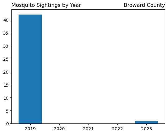
How many mosquito observations have been submitted to GLOBE Observer each year? We’ll make a bar plot to figure this out.

# Add a new column for year
data_county['MeasuredYear'] = data_county['MeasuredAt'].dt.year

# Make histogram of mosquito sightings each year
years = data_county[['SiteId', 'MeasuredYear']].groupby('MeasuredYear', as_index=False).count()
plt.bar(years['MeasuredYear'], years['SiteId'])
plt.title("Mosquito Sightings by Year", loc = 'left')
plt.title(county_name, loc = 'right')
plt.show()

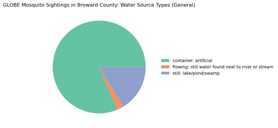
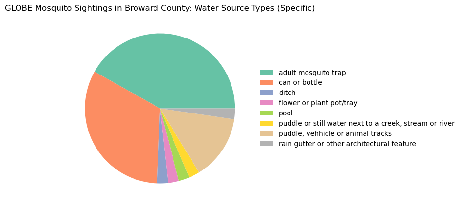
Let’s make a pie chart of the water source types (both general and specific) where mosquitoes were reported in this county.

types = data_county[['SiteId', 'WaterSourceType']].groupby('WaterSourceType', as_index=False).count()

plt.figure(figsize=(5, 5))
patches, texts = plt.pie(x = types['SiteId'],
                         colors = sns.color_palette('Set2'))
plt.title(f"GLOBE Mosquito Sightings in {county_name}: Water Source Types (General)")
plt.legend(patches, types['WaterSourceType'],
           loc = 'center left', bbox_to_anchor=(1, 0.5), frameon=False)
plt.show()

types = data_county[['SiteId', 'WaterSource']].groupby('WaterSource', as_index=False).count()

plt.figure(figsize=(5, 5))
patches, texts = plt.pie(x = types['SiteId'],
                         colors = sns.color_palette('Set2'))
plt.title(f"GLOBE Mosquito Sightings in {county_name}: Water Source Types (Specific)")
plt.legend(patches, types['WaterSource'],
           loc = 'center left', bbox_to_anchor=(1, 0.5), frameon=False)
plt.show()

Temperature and Land Use

The following code sets everything up needed for our analysis using Google Earth Engine.

from datetime import datetime
import numpy as np
from pylab import *
import folium
import ee
import geemap
import geopandas as gpd
ee.Authenticate()

# Write your project ID here, in quotes
ee.Initialize(project = "emerge-lessons")

def add_ee_layer(self, ee_image_object, vis_params, name):
    """Adds a method for displaying Earth Engine image tiles to folium map."""
    map_id_dict = ee.Image(ee_image_object).getMapId(vis_params)
    folium.raster_layers.TileLayer(
        tiles=map_id_dict['tile_fetcher'].url_format,
        attr='Map Data &copy; <a href="https://earthengine.google.com/">Google Earth Engine</a>',
        name=name,
        overlay=True,
        control=True
    ).add_to(self)

folium.Map.add_ee_layer = add_ee_layer

# Convert county boundaries to Earth Engine format
region = geemap.geopandas_to_ee(county)

# Zoom to the county
county_center = county.iloc[0].geometry.centroid

map = folium.Map([county_center.y, county_center.x], tiles="Cartodb dark_matter", zoom_start=10)

Map land surface temperature across the county.

First, define a date range. We will find the average temperature within this range. For this example, we will use June 2025. The start date is inclusive (meaning we’ll get data including that date) and the end date is exclusive (meaning we’ll get all dates leading up to, but not including, the end date).

start_date = "2025-06-01"
end_date = "2025-07-01"

The data comes from Google Earth Engine: MOD11A1.061 Terra Land Surface Temperature and Emissivity Daily Global 1km. The land surface temperature data are scaled, so to get the original temperature in Kelvin, the value needs to be multipled by 0.02. Then, this can be converted into degrees Celsius and Fahrenheit.

def to_fahrenheit(lst):
  celsius = lst * 0.02 - 273.15
  fahrenheit = celsius * 1.8 + 32
  return fahrenheit

def to_lst(fahrenheit):
  celsius = (fahrenheit - 32) / 1.8
  lst = (celsius + 273.15) / 0.02
  return lst

lst = (
    ee.ImageCollection('MODIS/061/MOD11A1')
      .filterDate(start_date, end_date)
      .select('LST_Day_1km')
      .mean()   # Can also use median() here to get the median instead of the average
      .clip(region)
)

colors = [
    '040274', '040281', '0502a3', '0502b8', '0502ce', '0502e6',
    '0602ff', '235cb1', '307ef3', '269db1', '30c8e2', '32d3ef',
    '3be285', '3ff38f', '86e26f', '3ae237', 'b5e22e', 'd6e21f',
    'fff705', 'ffd611', 'ffb613', 'ff8b13', 'ff6e08', 'ff500d',
    'ff0000', 'de0101', 'c21301', 'a71001', '911003'
]

lst_vis = {
    'min': to_lst(50), # 50 *F
    'max': to_lst(100), # 100 *F
    'palette': colors,
}

map.add_ee_layer(lst, lst_vis, "LST")

display(map)

Make this Notebook Trusted to load map: File -> Trust Notebook

Below is a colorbar that shows what the colors on the map represents: land surface temperature in degrees Fahrenheit.

plt.figure(figsize=(len(colors), 1))
plt.imshow([ [to_rgb(f'#{c}') for c in colors] ])

plt.text(-0.6, 0.1, '50 °F', va='center', ha='right', fontsize=24)
plt.text(len(colors) - 0.4, 0.1, '100 °F', va='center', ha='left', fontsize=24)

plt.axis('off')
plt.show()

Next, find the average temperature across the county.

mean_lst = lst.reduceRegion(reducer=ee.Reducer.mean(), geometry=region, scale=1000,
                              maxPixels=1e12).get('LST_Day_1km').getInfo()

print(f"The average temperature for {county_name} from {start_date} to {end_date} is {round(to_fahrenheit(mean_lst), 2)}°F")

The average temperature for Broward County from 2025-06-01 to 2025-07-01 is 87.67°F

See the land use and land cover in the county.

## Land Use

# Reset the map
map = folium.Map([county_center.y, county_center.x], tiles="Cartodb dark_matter", zoom_start=10)

# Define land cover color palette
palette = ['fbff97', 'e6558b', '004e2b', '9dbac5', 'a6976a', '1b1716']
visual = {'min': 1, 'max': 6, 'palette': palette}

landcover_1985 = (
    ee.ImageCollection('USFS/GTAC/LCMS/v2024-10')
      .filterDate('1985', '1986')
      .filter('study_area == "CONUS"')
      .first()
      .clip(region)
)

map.add_ee_layer(landcover_1985.select('Land_Use'), visual, '1985 Land Use')

landcover_2024 = (
    ee.ImageCollection('USFS/GTAC/LCMS/v2024-10')
      .filterDate('2024', '2025')
      .filter('study_area == "CONUS"')
      .first()
      .clip(region)
)

map.add_ee_layer(landcover_2024.select('Land_Use'), visual, '2024 Land Use')

folium.LayerControl(collapsed = False).add_to(map)
display(map)

Make this Notebook Trusted to load map: File -> Trust Notebook

\[\color{#fbff97}Agriculture\]

\[\color{#e6558b}Developed\]

\[\color{#004e2b}Forest\]

\[\color{#9dbac5}Other\]

\[\color{#a6976a}Rangeland or Pasture\]

We will create a function that calculates the percent of each type of land use and land cover in the county.

def land_stats(image, name, labels):
  count = image.select(name).reduceRegion(ee.Reducer.frequencyHistogram(), geometry=region, scale=30, maxPixels=1e12).getInfo()

  land_cover_counts = {}

  for key, value in labels.items():
      if key in count[name]:
          land_cover_counts[value] = count[name][key]

  total_pixels = sum([land_cover_counts[i] for i in land_cover_counts])

  for label, num in land_cover_counts.items():
    percent = round(100 * num / total_pixels, 1)
    if percent > 0:
      print(f"{label}: {percent}%")

land_use_labels = {'1': 'Agriculture',
                   '2': 'Developed',
                   '3': 'Forest',
                   '4': 'Other',
                   '5': 'Rangeland or Pasture',
                   '6': 'Non-Processing Area Mask'}

land_stats(landcover_1985, 'Land_Use', land_use_labels)

Agriculture: 4.5%
Developed: 19.6%
Forest: 8.5%
Other: 9.6%
Rangeland or Pasture: 55.8%
Non-Processing Area Mask: 2.0%

Now, we repeat for 2024.

land_stats(landcover_2024, 'Land_Use', land_use_labels)

Agriculture: 0.6%
Developed: 29.4%
Forest: 11.6%
Other: 15.2%
Rangeland or Pasture: 43.1%

## Land Cover

# Reset the map
map = folium.Map([county_center.y, county_center.x], tiles="Cartodb dark_matter", zoom_start=10)

palette = ['004e2b', '009344', '61bb46', 'acbb67', '8b8560', 'cafd4b', 'f89a1c', '8fa55f', 'bebb8e', 'e5e98a', 'ddb925', '893f54', 'e4f5fd', '00b6f0', '1b1716']
visual = {'min': 1, 'max': 15, 'palette': palette}

# Add land cover for 1985 and 2024
map.add_ee_layer(landcover_1985.select('Land_Cover'), visual, '1985 Land Cover')
map.add_ee_layer(landcover_2024.select('Land_Cover'), visual, '2024 Land Cover')

folium.LayerControl(collapsed = False).add_to(map)
display(map)

Make this Notebook Trusted to load map: File -> Trust Notebook

\[\color{#004e2b}Trees\]

\[\color{#61bb46}Shrubs \space and \space Trees Mix\]

\[\color{#acbb67}Grass/Forb/Herb \space and \space Trees Mix\]

\[\color{#8b8560}Barren \space and \space Trees Mix\]

\[\color{#f89a1c}Shrubs\]

\[\color{#8fa55f}Grass/Forb/Herb \space and \space Shrubs Mix\]

\[\color{#bebb8e}Barren \space and \space Shrubs Mix\]

\[\color{#e5e98a}Grass/Forb/Herb\]

\[\color{#ddb925}Barren \space and \space Grass/Forb/Herb Mix\]

\[\color{#893f54}Barren or Impervious\]

\[\color{#e4f5fd}Snow or Ice\]

Find the percent of each type of land cover.

land_cover_labels = {
    '1': 'Trees',
    '2': 'Tall Shrubs & Trees Mix (AK Only)',
    '3': 'Shrubs & Trees Mix',
    '4': 'Grass/Forb/Herb & Trees Mix',
    '5': 'Barren & Trees Mix',
    '6': 'Tall Shrubs (AK Only)',
    '7': 'Shrubs',
    '8': 'Grass/Forb/Herb & Shrubs Mix',
    '9': 'Barren & Shrubs Mix',
    '10': 'Grass/Forb/Herb',
    '11': 'Barren & Grass/Forb/Herb Mix',
    '12': 'Barren or Impervious',
    '13': 'Snow or Ice',
    '14': 'Water',
    '15': 'Non-Processing Area Mask'
}

land_stats(landcover_1985, 'Land_Cover', land_cover_labels)

Trees: 10.5%
Grass/Forb/Herb & Trees Mix: 1.2%
Grass/Forb/Herb & Shrubs Mix: 0.1%
Grass/Forb/Herb: 61.6%
Barren or Impervious: 16.6%
Water: 8.1%
Non-Processing Area Mask: 2.0%

land_stats(landcover_2024, 'Land_Cover', land_cover_labels)

Trees: 15.7%
Grass/Forb/Herb & Trees Mix: 1.2%
Grass/Forb/Herb & Shrubs Mix: 0.1%
Grass/Forb/Herb: 48.8%
Barren or Impervious: 19.9%
Water: 14.2%

Data:

• MOD11A1.061 Terra Land Surface Temperature and Emissivity Daily Global 1km

• USFS Landscape Change Monitoring System v2024.10 (CONUS and OCONUS)