
![]()
What is Coding?#
Intro to Python, Google Colab, and Data Science.
To run the code:
Make sure you have this notebook open in Google Colab. If you are starting from the digital textbook, click
Each block of code is called a cell. To run a cell, hover over it and click the arrow in the top left of the cell, or click inside of the cell and press Shift + Enter.
Note: When you run a block of code for the first time, Google Colab will say Warning: This notebook was not authored by Google. Please click Run Anyway.
A great feature of Google Colab is that you are able to write Python code and see the output directly on your browser. Let’s go through the basics below:
# This is a comment (added using a hashtag # at the start), used by programmers to explain their code
print("Hello World!")
# Comments do not impact how the code runs
Hello World!
Python Basics#
Python is a powerful tool for processing and analyzing data - perfect for this project. Let’s explore some of the basic functionality.
A variable can be used to store values calculated in expressions and then used for other calculations.
Defining variables is straightforward, but in good naming practice use an underscore (_) rather than a space.
# Setting up two variables
variable_one = 1
variable_two = 2

# Performing a calculation using those variables
variable_three = variable_one + variable_two

# Print the variable to see the result
print(variable_three)
3
There are different types of variables in Python. Here are the main variable types you may run into. Note: The spaces between the left and right parentheses are just to make it easier to see. You can remove the spaces or add more without impacting how the code runs
print(type( 100 ))
print(type( "Word" ))
print(type( 100.10 ))
print(type( True ))
print(type( [0, 1] ))
print(type( (0, 1) ))
print(type( {"Key": "Value"} ))
<class 'int'>
<class 'str'>
<class 'float'>
<class 'bool'>
<class 'list'>
<class 'tuple'>
<class 'dict'>
weather_forecast = "Hot"
type(weather_forecast)
str
daily_temperature = 85.0
type(daily_temperature)
float
You can redefine variables or convert their types. To redefine, you take the original variable and assign it a different value.
daily_temperature = "85.0"
type(daily_temperature)
str
updated_temperature = float(daily_temperature)
# We can confirm the type has changed by using the type() function again

type(updated_temperature)
float
So the value stays the same, but the variable type changes.
print(updated_temperature)
85.0
Functions are blocks of code that you use for a specific task that are easy to reuse.
We’ll define our first function in order to convert Fahrenheit to Celsius.
defis the keywordcelsius_to_fahris the function nametempis the parameter
def celsius_to_fahrenheit(temp):
    return 9 / 5 * temp + 32
To call a function, it’s the same as asking the terminal to print
freezing_point = celsius_to_fahrenheit(0)
print(f"The freezing point of water in Fahrenheit is: {freezing_point}")
The freezing point of water in Fahrenheit is: 32.0
You can also define a function using lambda. This helps us create small functions using just one line.
fahrenheit_to_celsius = lambda temp: (temp - 32) * 5 / 9
We can then use the lambda function the same as before.
freezing_point = fahrenheit_to_celsius(32)
print(f"The freezing point of water in Celsius is: {freezing_point}")
The freezing point of water in Celsius is: 0.0
Learn more about Python with these free resources:
Data Science Basics#
This section will provide an introduction to working with data in Python, including common libraries, loading data, and creating graphs.
Python has “libraries” that you can import, which expands the options we have with our code. Each library comes with many functions designed to accomplish specific tasks, like loading a dataset, performing calculations, making a chart, and more.
Import pandas, A popular library for processing and analyzing data.
import pandas as pd
Google Colab has pre-loaded datasets that anyone can use. Below, when we use pd.read_csv, we are using the Pandas library that we imported above.
data = pd.read_csv("sample_data/california_housing_test.csv")
Here, data is a dataframe that stores the data in memory. Run the code below to show the first 10 rows of the data. If we wrote data.head(), this will show 5 rows by default. If we just wrote data, this will show the first 5 rows and last 5 rows.
data.head(10)
| longitude | latitude | housing_median_age | total_rooms | total_bedrooms | population | households | median_income | median_house_value | |
|---|---|---|---|---|---|---|---|---|---|
| 0 | -122.05 | 37.37 | 27.0 | 3885.0 | 661.0 | 1537.0 | 606.0 | 6.6085 | 344700.0 |
| 1 | -118.30 | 34.26 | 43.0 | 1510.0 | 310.0 | 809.0 | 277.0 | 3.5990 | 176500.0 |
| 2 | -117.81 | 33.78 | 27.0 | 3589.0 | 507.0 | 1484.0 | 495.0 | 5.7934 | 270500.0 |
| 3 | -118.36 | 33.82 | 28.0 | 67.0 | 15.0 | 49.0 | 11.0 | 6.1359 | 330000.0 |
| 4 | -119.67 | 36.33 | 19.0 | 1241.0 | 244.0 | 850.0 | 237.0 | 2.9375 | 81700.0 |
| 5 | -119.56 | 36.51 | 37.0 | 1018.0 | 213.0 | 663.0 | 204.0 | 1.6635 | 67000.0 |
| 6 | -121.43 | 38.63 | 43.0 | 1009.0 | 225.0 | 604.0 | 218.0 | 1.6641 | 67000.0 |
| 7 | -120.65 | 35.48 | 19.0 | 2310.0 | 471.0 | 1341.0 | 441.0 | 3.2250 | 166900.0 |
| 8 | -122.84 | 38.40 | 15.0 | 3080.0 | 617.0 | 1446.0 | 599.0 | 3.6696 | 194400.0 |
| 9 | -118.02 | 34.08 | 31.0 | 2402.0 | 632.0 | 2830.0 | 603.0 | 2.3333 | 164200.0 |
See information about the data, including the columns, non-null count (non-null means not empty), and dtype (data type).
data.info()
<class 'pandas.core.frame.DataFrame'>
RangeIndex: 3000 entries, 0 to 2999
Data columns (total 9 columns):
 #   Column              Non-Null Count  Dtype
---  ------              --------------  -----
 0   longitude           3000 non-null   float64
 1   latitude            3000 non-null   float64
 2   housing_median_age  3000 non-null   float64
 3   total_rooms         3000 non-null   float64
 4   total_bedrooms      3000 non-null   float64
 5   population          3000 non-null   float64
 6   households          3000 non-null   float64
 7   median_income       3000 non-null   float64
 8   median_house_value  3000 non-null   float64
dtypes: float64(9)
memory usage: 211.1 KB
See the mean, standard deviation, minimum, and other qualities of each column in the data.
data.describe()
| longitude | latitude | housing_median_age | total_rooms | total_bedrooms | population | households | median_income | median_house_value | |
|---|---|---|---|---|---|---|---|---|---|
| count | 3000.000000 | 3000.00000 | 3000.000000 | 3000.000000 | 3000.000000 | 3000.000000 | 3000.00000 | 3000.000000 | 3000.00000 |
| mean | -119.589200 | 35.63539 | 28.845333 | 2599.578667 | 529.950667 | 1402.798667 | 489.91200 | 3.807272 | 205846.27500 |
| std | 1.994936 | 2.12967 | 12.555396 | 2155.593332 | 415.654368 | 1030.543012 | 365.42271 | 1.854512 | 113119.68747 |
| min | -124.180000 | 32.56000 | 1.000000 | 6.000000 | 2.000000 | 5.000000 | 2.00000 | 0.499900 | 22500.00000 |
| 25% | -121.810000 | 33.93000 | 18.000000 | 1401.000000 | 291.000000 | 780.000000 | 273.00000 | 2.544000 | 121200.00000 |
| 50% | -118.485000 | 34.27000 | 29.000000 | 2106.000000 | 437.000000 | 1155.000000 | 409.50000 | 3.487150 | 177650.00000 |
| 75% | -118.020000 | 37.69000 | 37.000000 | 3129.000000 | 636.000000 | 1742.750000 | 597.25000 | 4.656475 | 263975.00000 |
| max | -114.490000 | 41.92000 | 52.000000 | 30450.000000 | 5419.000000 | 11935.000000 | 4930.00000 | 15.000100 | 500001.00000 |
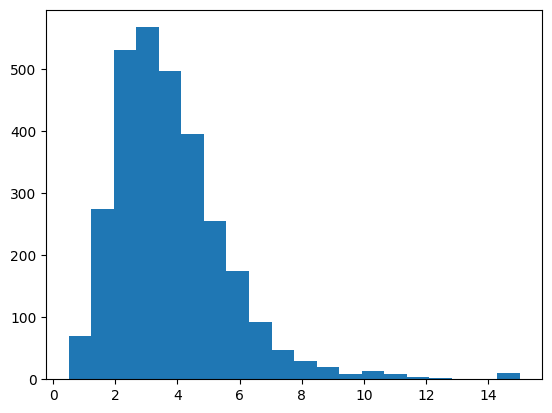
Import Matplotlib, a popular library for making visualizing data.
import matplotlib.pyplot as plt
plt.hist(data["median_income"], bins=20)
plt.show()
Import the GeoPandas library, useful for working with spatial data (any data with locations like addresses or coordinates).
import geopandas as gpd
geo_data = gpd.GeoDataFrame(
    data,
    geometry=gpd.points_from_xy(data.longitude, data.latitude),
    crs="EPSG:4326"
)

geo_data
| longitude | latitude | housing_median_age | total_rooms | total_bedrooms | population | households | median_income | median_house_value | geometry | |
|---|---|---|---|---|---|---|---|---|---|---|
| 0 | -122.05 | 37.37 | 27.0 | 3885.0 | 661.0 | 1537.0 | 606.0 | 6.6085 | 344700.0 | POINT (-122.05 37.37) |
| 1 | -118.30 | 34.26 | 43.0 | 1510.0 | 310.0 | 809.0 | 277.0 | 3.5990 | 176500.0 | POINT (-118.3 34.26) |
| 2 | -117.81 | 33.78 | 27.0 | 3589.0 | 507.0 | 1484.0 | 495.0 | 5.7934 | 270500.0 | POINT (-117.81 33.78) |
| 3 | -118.36 | 33.82 | 28.0 | 67.0 | 15.0 | 49.0 | 11.0 | 6.1359 | 330000.0 | POINT (-118.36 33.82) |
| 4 | -119.67 | 36.33 | 19.0 | 1241.0 | 244.0 | 850.0 | 237.0 | 2.9375 | 81700.0 | POINT (-119.67 36.33) |
| ... | ... | ... | ... | ... | ... | ... | ... | ... | ... | ... |
| 2995 | -119.86 | 34.42 | 23.0 | 1450.0 | 642.0 | 1258.0 | 607.0 | 1.1790 | 225000.0 | POINT (-119.86 34.42) |
| 2996 | -118.14 | 34.06 | 27.0 | 5257.0 | 1082.0 | 3496.0 | 1036.0 | 3.3906 | 237200.0 | POINT (-118.14 34.06) |
| 2997 | -119.70 | 36.30 | 10.0 | 956.0 | 201.0 | 693.0 | 220.0 | 2.2895 | 62000.0 | POINT (-119.7 36.3) |
| 2998 | -117.12 | 34.10 | 40.0 | 96.0 | 14.0 | 46.0 | 14.0 | 3.2708 | 162500.0 | POINT (-117.12 34.1) |
| 2999 | -119.63 | 34.42 | 42.0 | 1765.0 | 263.0 | 753.0 | 260.0 | 8.5608 | 500001.0 | POINT (-119.63 34.42) |
3000 rows × 10 columns
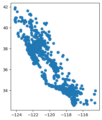
Make a simple map of the points.
geo_data.plot()
<Axes: >
Data Analysis Activity#
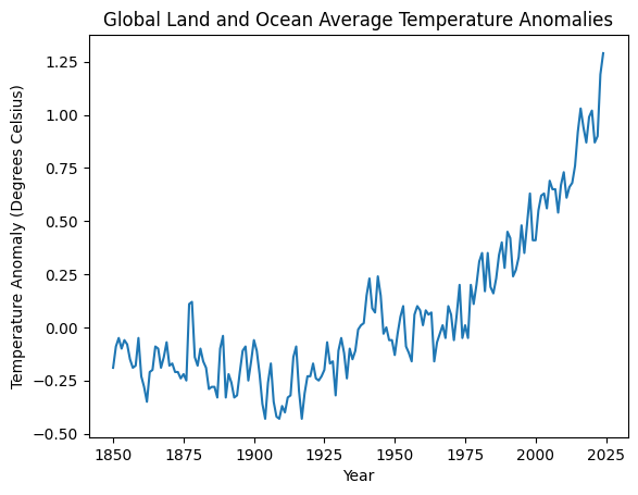
Data from NOAA”s Climate at a Glance Global Time Series
Title: Global Land and Ocean Average Temperature Anomalies
Units: Degrees Celsius
Base Period: 1901-2000
We can get data directly from the url (no need to download).
data = pd.read_csv("https://www.ncei.noaa.gov/access/monitoring/climate-at-a-glance/global/time-series/globe/tavg/land_ocean/ytd/12/1850-2025/data.csv",
                   skiprows=3) # Skip the first 3 rows because they state the title, units, and period of the data
data.head(10)
| Year | Anomaly | |
|---|---|---|
| 0 | 1850 | -0.19 |
| 1 | 1851 | -0.09 |
| 2 | 1852 | -0.05 |
| 3 | 1853 | -0.10 |
| 4 | 1854 | -0.06 |
| 5 | 1855 | -0.08 |
| 6 | 1856 | -0.15 |
| 7 | 1857 | -0.19 |
| 8 | 1858 | -0.18 |
| 9 | 1859 | -0.05 |
plt.plot(data["Year"], data["Anomaly"])

plt.title("Global Land and Ocean Average Temperature Anomalies")
plt.ylabel("Temperature Anomaly (Degrees Celsius)")
plt.xlabel("Year")
plt.show()
Let’s look at another dataset: Ambient Air Monitoring Sites in Florida - May 2023 from the Florida Department of Environmental Protection available through the Florida Geographic Data Library.
data = gpd.read_file('https://fgdl.org/zips/geospatial_data/archive/airmonitoring_may23.zip')
data.head()
| AGENCY | MANAGING_P | SITE_ID | COUNTY_FIP | COUNTY | SITE_NAME | CO | NO2 | O3 | PB | ... | LONGITUDE | LATITUDE | LAT_DD | LONG_DD | MGRS | GOOGLEMAP | DESCRIPT | FGDLAQDATE | AUTOID | geometry | |
|---|---|---|---|---|---|---|---|---|---|---|---|---|---|---|---|---|---|---|---|---|---|
| 0 | 867.0 | LOCAL - PINELLAS CNTY DEM | L103-0012 | 103.0 | PINELLAS | WOODLAWN | 0.0 | 0.0 | 0.0 | 0.0 | ... | -82.659265 | 27.784749 | 27.784749 | -82.659265 | 17RLL3652074461 | https://www.google.com/maps/place/17RLL3652074461 | PINELLAS (WOODLAWN) | 2023-06-27 | 71 | POINT (531854.993 420607.238) |
| 1 | 867.0 | LOCAL - PINELLAS CNTY DEM | L103-0018 | 103.0 | PINELLAS | AZALEA PARK | 0.0 | 1.0 | 1.0 | 0.0 | ... | -82.739875 | 27.785866 | 27.785866 | -82.739875 | 17RLL2857974695 | https://www.google.com/maps/place/17RLL2857974695 | PINELLAS (AZALEA PARK) | 2023-06-27 | 72 | POINT (523926.446 420647.656) |
| 2 | 867.0 | LOCAL - PINELLAS CNTY DEM | L103-0023 | 103.0 | PINELLAS | DERBY LANE | 0.0 | 0.0 | 0.0 | 0.0 | ... | -82.623153 | 27.863635 | 27.863635 | -82.623153 | 17RLL4019483154 | https://www.google.com/maps/place/17RLL4019483154 | PINELLAS (DERBY LANE) | 2023-06-27 | 73 | POINT (535308.445 429406.36) |
| 3 | 867.0 | LOCAL - PINELLAS CNTY DEM | L103-0026 | 103.0 | PINELLAS | SKYVIEW DRIVE | 0.0 | 0.0 | 0.0 | 0.0 | ... | -82.714600 | 27.850000 | 27.850000 | -82.714600 | 17RLL3116981766 | https://www.google.com/maps/place/17RLL3116981766 | PINELLAS (SKYVIEW DRIVE) | 2023-06-27 | 74 | POINT (526337.746 427795.197) |
| 4 | 867.0 | LOCAL - PINELLAS CNTY DEM | L103-0027 | 103.0 | PINELLAS | SAWGRASS LAKE PARK | 1.0 | 1.0 | 0.0 | 0.0 | ... | -82.665251 | 27.834400 | 27.834400 | -82.665251 | 17RLL3600579971 | https://www.google.com/maps/place/17RLL3600579971 | PINELLAS (SAWGRASS LAKE PARK) | 2023-06-27 | 75 | POINT (531206.635 426114.408) |
5 rows × 29 columns
data.plot()
<Axes: >

Let’s update the design of the map using another Python library, contextily. We need to write pip install contextily to manually install the library first. This is because Google Colab does not include contextily by default, unlike the libraries we have used so far (pandas, geopandas, matplotlib).
!pip install contextily
import contextily as cx
First, we use .to_crs(epsg=3857) to set the data to a coordinate reference system that is consistent with the basemap (the map in the background) that we want to add.
ax = data.to_crs(epsg=3857).plot(color="orange",
                                    edgecolor="black",
                                    markersize=30)
cx.add_basemap(ax)
ax.set_title("Ambient Air Monitoring Sites in Florida")
plt.show()

That’s it for this section! Continue to the next section to see how to use Google Earth Engine in Python to view satellite images and other Earth data.