

Mosquito & Land Cover Stats#
This lesson shows how to investigate the GLOBE data, calculate statistics, and create charts & maps.
import pandas as pd
pd.set_option("display.max_columns", None)
import geopandas as gpd
import matplotlib.pyplot as plt
import seaborn as sns
import folium
Mosquito#
Let’s load the data directly from the link (no need to download anything to your computer).
mosquito = gpd.read_file('https://github.com/geo-di-lab/emerge-lessons/raw/refs/heads/main/docs/data/globe_mosquito.zip')
mosquito.head()
| CountryCode | CountryName | Elevation | AbdomenCloseupPhotoUrls | BreedingGroundEliminated | Comments | DataSource | ExtraData | Genus | GlobeTeams | LarvaFullBodyPhotoUrls | LarvaeCount | LastIdentifyStage | LocationAccuracyM | LocationMethod | MeasuredAt | MeasurementElevation | MeasurementLatitude | MeasurementLongitude | MosquitoAdults | MosquitoEggs | MosquitoHabitatMapperId | MosquitoPupae | Species | Userid | WaterSource | WaterSourcePhotoUrls | WaterSourceType | OrganizationId | OrganizationName | Protocol | SiteId | SiteName | MeasuredDate | LarvaeCountProcessed | geometry | |
|---|---|---|---|---|---|---|---|---|---|---|---|---|---|---|---|---|---|---|---|---|---|---|---|---|---|---|---|---|---|---|---|---|---|---|---|---|
| 0 | BRA | Brazil | 6.3 | NaN | false | NaN | GLOBE Observer App | LarvaeVisibleNo | NaN | [COLUNSLZ] | NaN | 0 | NaN | 13 | automatic | 2024-12-31 17:16:00 | 0 | -2.5617 | -44.2657 | NaN | NaN | 46287 | false | NaN | 137422629 | ovitrap | https://data.globe.gov/system/photos/2024/12/3... | container: artificial | 17459532 | Brazil Citizen Science | mosquito_habitat_mapper | 371514 | 23MNT816168 | 2024-12-31 | 0.0 | POINT (-44.26597 -2.56197) |
| 1 | BRA | Brazil | 6.3 | NaN | false | NaN | GLOBE Observer App | LarvaeVisibleNo | NaN | [COLUNSLZ] | NaN | 0 | NaN | 13 | automatic | 2024-12-31 17:20:00 | 0 | -2.5617 | -44.2657 | NaN | NaN | 46290 | false | NaN | 137422629 | ovitrap | https://data.globe.gov/system/photos/2024/12/3... | container: artificial | 17459532 | Brazil Citizen Science | mosquito_habitat_mapper | 371514 | 23MNT816168 | 2024-12-31 | 0.0 | POINT (-44.26597 -2.56197) |
| 2 | BRA | Brazil | 7.4 | NaN | true | NaN | GLOBE Observer App | LarvaeVisibleNo | NaN | [COLUNSLZ] | NaN | 0 | NaN | 51 | automatic | 2024-12-31 22:32:00 | 0 | -2.5163 | -44.3023 | NaN | NaN | 46482 | false | NaN | 137420190 | cement, metal or plastic tank | NaN | container: artificial | 17459532 | Brazil Citizen Science | mosquito_habitat_mapper | 372864 | 23MNT775218 | 2024-12-31 | 0.0 | POINT (-44.30288 -2.51676) |
| 3 | BRA | Brazil | 20.6 | NaN | true | NaN | GLOBE Observer App | LarvaeVisibleNo | NaN | [COLUNSLZ] | NaN | 0 | NaN | 66 | automatic | 2024-12-31 00:05:00 | 0 | -2.8639 | -44.0549 | NaN | NaN | 46203 | false | NaN | 137419937 | can or bottle | NaN | container: artificial | 17459532 | Brazil Citizen Science | mosquito_habitat_mapper | 373085 | 23MPS050834 | 2024-12-31 | 0.0 | POINT (-44.05526 -2.86396) |
| 4 | BRA | Brazil | 20.6 | NaN | true | NaN | GLOBE Observer App | LarvaeVisibleNo | NaN | [COLUNSLZ] | NaN | 0 | NaN | 28 | automatic | 2024-12-31 00:23:00 | 0 | -2.8639 | -44.0550 | NaN | NaN | 46223 | false | NaN | 137419937 | lake | NaN | still: lake/pond/swamp | 17459532 | Brazil Citizen Science | mosquito_habitat_mapper | 373085 | 23MPS050834 | 2024-12-31 | 0.0 | POINT (-44.05526 -2.86396) |
See the list of columns:
mosquito.info()
<class 'geopandas.geodataframe.GeoDataFrame'>
RangeIndex: 43012 entries, 0 to 43011
Data columns (total 36 columns):
# Column Non-Null Count Dtype
--- ------ -------------- -----
0 CountryCode 42928 non-null str
1 CountryName 42928 non-null str
2 Elevation 43012 non-null str
3 AbdomenCloseupPhotoUrls 874 non-null str
4 BreedingGroundEliminated 42951 non-null str
5 Comments 4002 non-null str
6 DataSource 43012 non-null str
7 ExtraData 12448 non-null str
8 Genus 4364 non-null str
9 GlobeTeams 16259 non-null str
10 LarvaFullBodyPhotoUrls 8632 non-null str
11 LarvaeCount 24691 non-null str
12 LastIdentifyStage 29911 non-null str
13 LocationAccuracyM 13814 non-null str
14 LocationMethod 18205 non-null str
15 MeasuredAt 43012 non-null datetime64[ms]
16 MeasurementElevation 42995 non-null str
17 MeasurementLatitude 42995 non-null float64
18 MeasurementLongitude 42995 non-null float64
19 MosquitoAdults 16852 non-null str
20 MosquitoEggs 16859 non-null str
21 MosquitoHabitatMapperId 43012 non-null str
22 MosquitoPupae 41210 non-null str
23 Species 1155 non-null str
24 Userid 43012 non-null str
25 WaterSource 43012 non-null str
26 WaterSourcePhotoUrls 34302 non-null str
27 WaterSourceType 43012 non-null str
28 OrganizationId 42928 non-null str
29 OrganizationName 42928 non-null str
30 Protocol 43012 non-null str
31 SiteId 43012 non-null str
32 SiteName 43012 non-null str
33 MeasuredDate 43012 non-null str
34 LarvaeCountProcessed 24688 non-null float64
35 geometry 43012 non-null geometry
dtypes: datetime64[ms](1), float64(3), geometry(1), str(31)
memory usage: 25.4 MB
How many rows are in the dataset?
len(mosquito)
43012
There were 43,012 citizen science contributions from 2018 to 2024. Now, let’s see the number of countries where people submitted data.
len(mosquito['CountryCode'].unique())
95
Let’s see the types of the habitats (water sources) the citizen scientists recorded.
# Broader water source types
mosquito['WaterSourceType'].value_counts()
WaterSourceType
container: artificial 33167
still: lake/pond/swamp 6277
container: natural 2202
flowing: still water found next to river or stream 1366
Name: count, dtype: int64
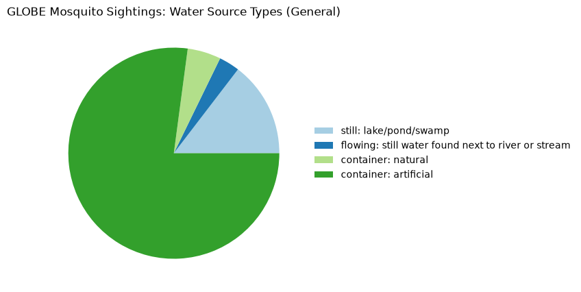
These are the general types of water sources that citizen scientists reported to NASA. It looks like most data were collected about artificial containers. Let’s see some of the more specific types in the other column:
# More specific water source types
mosquito['WaterSource'].value_counts()
WaterSource
cement, metal or plastic tank 7528
dish or pot 4102
well or cistern 2790
jar 2399
fountain or bird bath 2350
ovitrap 2243
adult mosquito trap 2073
pond 2029
other 1915
can or bottle 1888
ditch 1886
tire 1885
animal trough or water bowl 1177
puddle or still water next to a creek, stream or river 993
flower or plant pot/tray 932
trash container 882
plant clumps (bamboo etc) 768
puddle, vehhicle or animal tracks 644
tree holes 571
public works - culvert, bridge, road 570
discarded: other 511
puddle, vehicle or animal tracks 475
swamp or wetland 467
plant husk (areca, coconut etc) 453
lake 415
rain gutter or other architectural feature 277
estuary 148
pool 128
old car or boat 123
reservoir 112
grill or outdoor appliance 108
refrigerator drainage 69
animal shell (tortoise, mollusk etc) 65
bay or ocean 36
Name: count, dtype: int64
Let’s make a pie chart using the broader column, WaterSourceType
# Here are some options for color palettes
display(sns.color_palette(palette='Set2'))
display(sns.color_palette(palette='twilight_shifted'))
display(sns.color_palette(palette='Paired'))
# Pie chart of water types
types = (mosquito[['SiteId', 'WaterSourceType']]
.groupby('WaterSourceType', as_index=False).count()
.sort_values(by='WaterSourceType', ascending=False))
plt.figure(figsize=(5, 5))
patches, texts = plt.pie(x = types['SiteId'],
colors = sns.color_palette('Paired'))
plt.title("GLOBE Mosquito Sightings: Water Source Types (General)")
plt.legend(patches, types['WaterSourceType'],
loc = 'center left', bbox_to_anchor=(1, 0.5), frameon=False)
plt.show()
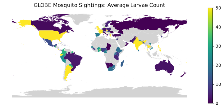
What is the average larvae count by country?
mosquito_avg = mosquito.groupby('CountryCode')['LarvaeCountProcessed'].mean()
mosquito_avg
CountryCode
ARE 5.000000
ARG 116.108108
AUS 2.500000
BEL NaN
BEN 38.598198
...
UKR NaN
URY 0.043478
USA 667.935961
VNM 22.686567
ZAF 17.800000
Name: LarvaeCountProcessed, Length: 94, dtype: float64
Let’s make a map showing the larvae count by country. The country boundaries (generalized) are from Esri, Garmin, and U.S. Central Intelligence Agency (The World Factbook). The boundaries are generalized to allow data processing and visualizations to load faster. The ISO alpha-3 codes come from the World Countries layer from Esri, Garmin, U.S. Central Intelligence Agency (The World Factbook), and International Organization for Standardization (ISO).
countries = gpd.read_file('https://github.com/geo-di-lab/emerge-lessons/raw/refs/heads/main/docs/data/world_countries_general.geojson').to_crs(epsg=4326)
mosquito_avg = countries.merge(mosquito_avg, left_on='iso3', right_on='CountryCode', how='left')
fig, ax = plt.subplots(figsize = (10, 4))
mosquito_avg.plot(column = 'LarvaeCountProcessed', cmap = 'viridis',
legend = True, vmin = 0, vmax = 50, ax = ax,
missing_kwds = {'color': 'lightgrey'})
plt.title('GLOBE Mosquito Sightings: Average Larvae Count')
ax.axis('off')
plt.show()
Now, we’ll make an interactive map showing total GLOBE observations by country.
mosquito_obs = mosquito.groupby('CountryCode').size() \
.reset_index(name='GLOBE_Observations')
mosquito_obs = countries.merge(mosquito_obs, left_on='iso3', right_on='CountryCode', how='left')
We will build both interactive maps in this lesson the same way, so we’ll write the map code once as a reusable function. The function colors each country by its number of observations, adds a legend that lists the range for every color, and shows a pop-up when you hover over a country.
# The color scheme (yellow-green-blue) and the cutoffs between colors
BINS = [1, 50, 100, 500, 1000, 5000, 10000, 20000, 35000]
COLORS = ['#ffffd9', '#edf8b1', '#c7e9b4', '#7fcdbb', '#41b6c4', '#1d91c0', '#225ea8', '#0c2c84']
NO_DATA = '#e8e8e8'
def observation_color(value):
"""Pick the color for a country based on its number of observations."""
if pd.isna(value):
return NO_DATA
for color, upper in zip(COLORS, BINS[1:]):
if value < upper:
return color
return COLORS[-1]
def make_legend(title):
"""Create legend for the map."""
rows = ""
for i, color in enumerate(COLORS):
low, high = BINS[i], BINS[i + 1]
label = f"{low:,} – {high - 1:,}" if i < len(COLORS) - 1 else f"{low:,}+"
rows += (f"<div style='margin:2px 0'><span style='display:inline-block;width:20px;height:13px;"
f"background:{color};border:1px solid #999;vertical-align:-2px'></span> {label}</div>")
rows += (f"<div style='margin:2px 0'><span style='display:inline-block;width:20px;height:13px;"
f"background:{NO_DATA};border:1px solid #999;vertical-align:-2px'></span> No data</div>")
return folium.Element(f"""
<div style="position:fixed; bottom:25px; left:15px; z-index:9999; background:white;
padding:10px 14px; border:1px solid #bbb; border-radius:6px;
box-shadow:0 1px 5px rgba(0,0,0,.3); font-family:Helvetica,Arial,sans-serif;
font-size:13px; color:#222; line-height:1.4;">
<div style="font-weight:bold; margin-bottom:6px;">{title}</div>
{rows}
</div>""")
def observation_map(data, tooltip_fields, tooltip_aliases, legend_title):
"""Make an interactive map of GLOBE observations by country."""
data = data.copy()
# Format the counts and say "No data" instead of showing an empty value
data['Observations'] = data['GLOBE_Observations'].apply(
lambda value: f"{value:,.0f}" if pd.notna(value) else "No data")
for field in tooltip_fields:
data[field] = data[field].fillna("No data")
map = folium.Map(location=[20, 0], zoom_start=2, min_zoom=2, tiles=None, max_bounds=True)
# Add Esri's light gray basemap
folium.TileLayer(
tiles="https://server.arcgisonline.com/ArcGIS/rest/services/Canvas/World_Light_Gray_Base/MapServer/tile/{z}/{y}/{x}",
attr="Tiles © Esri — Esri, DeLorme, NAVTEQ",
name="Light Gray Canvas",
no_wrap=True,
bounds=[[-85, -180], [85, 180]],
).add_to(map)
# Add GLOBE data with observation counts
folium.GeoJson(
data,
style_function=lambda feature: {
'fillColor': observation_color(feature['properties']['GLOBE_Observations']),
'color': 'white',
'weight': 0.7,
'fillOpacity': 0.85,
},
highlight_function=lambda feature: {'weight': 2.5, 'color': '#333', 'fillOpacity': 0.95},
tooltip=folium.GeoJsonTooltip(
fields=tooltip_fields,
aliases=tooltip_aliases,
sticky=True,
style=("background-color:white; border:1px solid #999; border-radius:4px; "
"box-shadow:0 1px 4px rgba(0,0,0,.3); padding:6px 8px; font-size:13px;"),
),
).add_to(map)
map.get_root().html.add_child(
folium.Element("<style>.leaflet-container{background:#f4f6f8;}</style>"))
map.get_root().html.add_child(make_legend(legend_title))
return map
map = observation_map(
mosquito_obs,
tooltip_fields=['name', 'Observations'],
tooltip_aliases=['Country:', 'Observations:'],
legend_title="GLOBE Mosquito Observations",
)
display(map)
Land Cover#
Load the land cover data directly from the link.
land_cover = gpd.read_file('https://github.com/geo-di-lab/emerge-lessons/raw/refs/heads/main/docs/data/globe_land_cover.zip')
land_cover.head()
| CountryCode | CountryName | Elevation | DataSource | DownwardCaption | DownwardExtraData | DownwardPhotoUrl | DryGround | EastCaption | EastClassifications | EastExtraData | EastPhotoUrl | Feature1Caption | Feature1ExtraData | Feature1PhotoUrl | Feature2Caption | Feature2ExtraData | Feature2PhotoUrl | Feature3Caption | Feature3ExtraData | Feature3PhotoUrl | Feature4Caption | Feature4ExtraData | Feature4PhotoUrl | FieldNotes | GlobeTeams | LandCoverId | LeavesOnTrees | LocationAccuracyM | LocationMethod | MeasuredAt | MeasurementElevation | MeasurementLatitude | MeasurementLongitude | MucCode | MucDescription | MucDetails | Muddy | NorthCaption | NorthClassifications | NorthExtraData | NorthPhotoUrl | RainingSnowing | SnowIce | SouthCaption | SouthClassifications | SouthExtraData | SouthPhotoUrl | StandingWater | UpwardCaption | UpwardExtraData | UpwardPhotoUrl | Userid | WestCaption | WestClassifications | WestExtraData | WestPhotoUrl | OrganizationId | OrganizationName | Protocol | SiteId | SiteName | MeasuredDate | geometry | |
|---|---|---|---|---|---|---|---|---|---|---|---|---|---|---|---|---|---|---|---|---|---|---|---|---|---|---|---|---|---|---|---|---|---|---|---|---|---|---|---|---|---|---|---|---|---|---|---|---|---|---|---|---|---|---|---|---|---|---|---|---|---|---|---|---|
| 0 | ITA | Italy | 489.2 | GLOBE Observer App | NaN | NaN | https://data.globe.gov/system/photos/2024/12/3... | true | NaN | NaN | NaN | https://data.globe.gov/system/photos/2024/12/3... | Snag C. sativa, 40 cm, cl 2, #01 #04 #12 | ((compassData.heading: 182, compassData.horizo... | https://data.globe.gov/system/photos/2024/12/3... | Log 70 cm, C. sativa, cl 2, #04 #01 #12 | ((compassData.heading: 182, compassData.horizo... | https://data.globe.gov/system/photos/2024/12/3... | Stump of C. sativa 230 cm | ((compassData.heading: null, compassData.horiz... | https://data.globe.gov/system/photos/2024/12/3... | NaN | NaN | NaN | Old Coppice of Castanea sativa | [Conservazione Natura Universita Tuscia] | 78608 | false | 8 | automatic | 2024-12-31 15:07:00.000 | 492.4 | 42.1818 | 12.1825 | NaN | NaN | false | NaN | NaN | NaN | https://data.globe.gov/system/photos/2024/12/3... | false | false | NaN | NaN | NaN | https://data.globe.gov/system/photos/2024/12/3... | false | NaN | NaN | https://data.globe.gov/system/photos/2024/12/3... | 128342138 | NaN | NaN | NaN | https://data.globe.gov/system/photos/2024/12/3... | 17453129 | Italy Citizen Science | land_covers | 376869 | 33TTG673738 | 2024-12-31 | POINT (12.18229 42.18175) | |
| 1 | MDG | Madagascar | 1350.1 | GLOBE Observer App | NaN | NaN | https://data.globe.gov/system/photos/2024/12/3... | true | NaN | 90% MUC 01 (n) [Trees, Closely Spaced, Evergre... | NaN | https://data.globe.gov/system/photos/2024/12/3... | NaN | NaN | NaN | NaN | NaN | NaN | NaN | NaN | NaN | NaN | NaN | NaN | Arbres plantés par l'équipe GLOBE avec la comm... | [Africa 2024 Regional Meeting, Coordinating Of... | 77695 | true | 10 | automatic | 2024-12-31 11:29:00.000 | 1340.6 | -18.7576 | 47.5615 | M01 | Trees, Closely Spaced, Evergreen - Needle Leaved | n | false | NaN | 90% MUC 01 (n) [Trees, Closely Spaced, Evergre... | NaN | https://data.globe.gov/system/photos/2024/12/3... | false | false | NaN | 90% MUC 01 (n) [Trees, Closely Spaced, Evergre... | NaN | https://data.globe.gov/system/photos/2024/12/3... | false | NaN | NaN | https://data.globe.gov/system/photos/2024/12/3... | 2538037 | NaN | 90% MUC 01 (n) [Trees, Closely Spaced, Evergre... | NaN | https://data.globe.gov/system/photos/2024/12/3... | 6508873 | Madagascar GLOBE v-School | land_covers | 373647 | 38KQE700240 | 2024-12-31 | POINT (47.56096 -18.75807) |
| 2 | MDG | Madagascar | 1324.7 | GLOBE Observer App | NaN | NaN | https://data.globe.gov/system/photos/2024/12/3... | true | NaN | 60% MUC 93 [Urban, Roads and Parking] | NaN | https://data.globe.gov/system/photos/2024/12/3... | NaN | NaN | NaN | NaN | NaN | NaN | NaN | NaN | NaN | NaN | NaN | NaN | NaN | [Africa 2024 Regional Meeting, Coordinating Of... | 77691 | true | 10 | automatic | 2024-12-31 12:07:00.000 | 1324.8 | -18.7944 | 47.5799 | M93 | Urban, Roads and Parking | false | NaN | 60% MUC 93 [Urban, Roads and Parking] | NaN | https://data.globe.gov/system/photos/2024/12/3... | false | false | NaN | 60% MUC 93 [Urban, Roads and Parking] | NaN | https://data.globe.gov/system/photos/2024/12/3... | false | NaN | NaN | https://data.globe.gov/system/photos/2024/12/3... | 2538037 | NaN | 60% MUC 93 [Urban, Roads and Parking] | NaN | https://data.globe.gov/system/photos/2024/12/3... | 6508873 | Madagascar GLOBE v-School | land_covers | 373642 | 38KQE719199 | 2024-12-31 | POINT (47.57953 -18.79484) | |
| 3 | USA | United States | 182.2 | GLOBE Data Entry Site Definition | NaN | NaN | NaN | NaN | NaN | NaN | NaN | NaN | NaN | NaN | NaN | NaN | NaN | NaN | NaN | NaN | NaN | NaN | NaN | NaN | NaN | NaN | 77689 | NaN | NaN | NaN | 2024-12-31 16:12:03.111 | NaN | NaN | NaN | M4 | Herbaceous Vegetation | NaN | NaN | NaN | NaN | NaN | NaN | NaN | NaN | NaN | NaN | NaN | NaN | NaN | NaN | NaN | NaN | NaN | NaN | NaN | NaN | NaN | 52107 | Crestwood High School | land_covers | 373628 | Hillcrest Elementary Trail | 2024-12-31 | POINT (-83.27705 42.3465) |
| 4 | GRC | Greece | 3.0 | GLOBE Observer App | NaN | NaN | https://data.globe.gov/system/photos/2024/12/3... | true | NaN | 90% MUC 91 [Urban, Residential Property]; 10% ... | NaN | https://data.globe.gov/system/photos/2024/12/3... | NaN | NaN | NaN | NaN | NaN | NaN | NaN | NaN | NaN | NaN | NaN | NaN | NaN | [tinycore lab, tinycorelab] | 77683 | false | NaN | manual | 2024-12-31 11:45:00.000 | 3.2 | 37.939 | 23.697 | M91 | Urban, Residential Property | false | NaN | 90% MUC 91 [Urban, Residential Property]; 10% ... | NaN | https://data.globe.gov/system/photos/2024/12/3... | false | false | NaN | 20% MUC 91 [Urban, Residential Property]; 80% ... | NaN | https://data.globe.gov/system/photos/2024/12/3... | false | NaN | NaN | https://data.globe.gov/system/photos/2024/12/3... | 65209921 | NaN | 10% MUC 91 [Urban, Residential Property]; 90% ... | NaN | https://data.globe.gov/system/photos/2024/12/3... | 6508393 | Greece GLOBE v-School | land_covers | 373613 | 34SGH370024 | 2024-12-31 | POINT (23.6969 37.9383) |
land_cover.info()
<class 'geopandas.geodataframe.GeoDataFrame'>
RangeIndex: 50783 entries, 0 to 50782
Data columns (total 64 columns):
# Column Non-Null Count Dtype
--- ------ -------------- -----
0 CountryCode 48376 non-null str
1 CountryName 48376 non-null str
2 Elevation 50783 non-null str
3 DataSource 50783 non-null str
4 DownwardCaption 22409 non-null str
5 DownwardExtraData 22405 non-null str
6 DownwardPhotoUrl 39585 non-null str
7 DryGround 43453 non-null str
8 EastCaption 23641 non-null str
9 EastClassifications 14314 non-null str
10 EastExtraData 23636 non-null str
11 EastPhotoUrl 42406 non-null str
12 Feature1Caption 337 non-null str
13 Feature1ExtraData 1359 non-null str
14 Feature1PhotoUrl 1360 non-null str
15 Feature2Caption 156 non-null str
16 Feature2ExtraData 676 non-null str
17 Feature2PhotoUrl 676 non-null str
18 Feature3Caption 96 non-null str
19 Feature3ExtraData 448 non-null str
20 Feature3PhotoUrl 448 non-null str
21 Feature4Caption 77 non-null str
22 Feature4ExtraData 337 non-null str
23 Feature4PhotoUrl 337 non-null str
24 FieldNotes 21043 non-null str
25 GlobeTeams 23723 non-null str
26 LandCoverId 50783 non-null str
27 LeavesOnTrees 43453 non-null str
28 LocationAccuracyM 36355 non-null str
29 LocationMethod 43453 non-null str
30 MeasuredAt 50783 non-null datetime64[ms]
31 MeasurementElevation 43400 non-null str
32 MeasurementLatitude 43400 non-null str
33 MeasurementLongitude 43400 non-null str
34 MucCode 21835 non-null str
35 MucDescription 21832 non-null str
36 MucDetails 43453 non-null str
37 Muddy 43453 non-null str
38 NorthCaption 23929 non-null str
39 NorthClassifications 14345 non-null str
40 NorthExtraData 23929 non-null str
41 NorthPhotoUrl 42773 non-null str
42 RainingSnowing 43453 non-null str
43 SnowIce 43453 non-null str
44 SouthCaption 23509 non-null str
45 SouthClassifications 14311 non-null str
46 SouthExtraData 23507 non-null str
47 SouthPhotoUrl 42292 non-null str
48 StandingWater 43453 non-null str
49 UpwardCaption 22905 non-null str
50 UpwardExtraData 22898 non-null str
51 UpwardPhotoUrl 40348 non-null str
52 Userid 43453 non-null str
53 WestCaption 23472 non-null str
54 WestClassifications 14284 non-null str
55 WestExtraData 23482 non-null str
56 WestPhotoUrl 42197 non-null str
57 OrganizationId 48377 non-null str
58 OrganizationName 48377 non-null str
59 Protocol 50783 non-null str
60 SiteId 50783 non-null str
61 SiteName 50783 non-null str
62 MeasuredDate 50783 non-null str
63 geometry 50783 non-null geometry
dtypes: datetime64[ms](1), geometry(1), str(62)
memory usage: 69.0 MB
len(land_cover)
50783
There are slightly more observations submitted for GLOBE Land Cover (50,766 observations) than Mosquito Habitat Mapper.
len(land_cover['CountryCode'].unique())
98
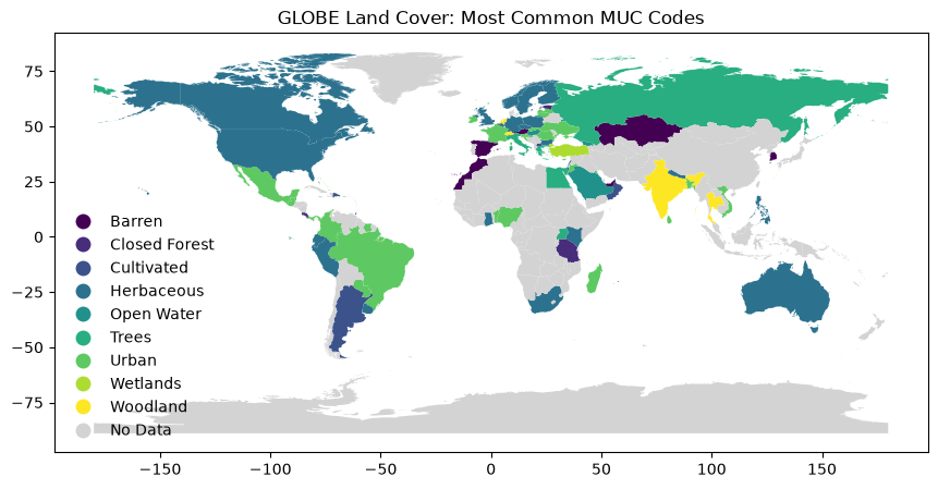
A helpful part of the land cover dataset is the MUC classifications. MUC, Modified UNESCO Classification, is a classification system with different land use types.
# Let's see the different MUC codes
len(land_cover['MucCode'].unique())
154
# What are the most common MUC codes by country?
muc = land_cover.groupby('CountryCode')['MucDescription'] \
.apply(lambda x: x.value_counts().idxmax() if not x.value_counts().empty else None).reset_index(name='MucDescription')
# Add a column for the number of the MUC code
muc['Count'] = land_cover.groupby('CountryCode')['MucDescription'] \
.apply(lambda x: x.value_counts().max()).values
# Add a column for the total number of GLOBE observations
muc['GLOBE_Observations'] = land_cover.groupby('CountryCode').size().values
muc
| CountryCode | MucDescription | Count | GLOBE_Observations | |
|---|---|---|---|---|
| 0 | ARE | Barren, Bare Rock | 1.0 | 25 |
| 1 | ARG | Cultivated Land, Non-Agriculture, Parks and At... | 135.0 | 1109 |
| 2 | ARM | NaN | NaN | 1 |
| 3 | AUS | Herbaceous/Grassland, Short Grass | 8.0 | 346 |
| 4 | AUT | Barren, Dirt/Other | 1.0 | 10 |
| ... | ... | ... | ... | ... |
| 92 | UKR | Urban, Other | 8.0 | 224 |
| 93 | URY | Herbaceous Vegetation | 8.0 | 35 |
| 94 | USA | Herbaceous/Grassland, Short Grass | 2788.0 | 30122 |
| 95 | VNM | Urban, Commercial Property | 6.0 | 56 |
| 96 | ZAF | Herbaceous/Grassland, Short Grass | 4.0 | 107 |
97 rows × 4 columns
# We can check that this is correct by checking one of the countries
print('Count of most common MUC:', len(land_cover[(land_cover['CountryCode'] == 'USA') &
(land_cover['MucDescription'] == 'Herbaceous/Grassland, Short Grass')]))
print('Total GLOBE Observations:', len(land_cover[(land_cover['CountryCode'] == 'USA')]))
Count of most common MUC: 2788
Total GLOBE Observations: 30122
We can see that the number of rows matches the number in the dataset above, so we know this was calculated correctly.
muc = countries.merge(muc, left_on='iso3', right_on='CountryCode', how='left')
Some of the MUC descriptions are similar, so we’ll group by the general categories of Barren, Closed Forest, Cultivated, and others below.
muc_list = ['Barren', 'Closed Forest', 'Cultivated', 'Herbaceous', 'Open Water', 'Trees', 'Urban', 'Wetlands', 'Woodland']
for muc_code in muc_list:
muc.loc[muc['MucDescription'].str.contains(muc_code, na=False), 'MucDescriptionShort'] = muc_code
fig, ax = plt.subplots(figsize = (11, 5))
muc.plot(column = 'MucDescriptionShort', cmap = 'viridis',
legend = True, ax = ax,
missing_kwds = {'color': 'lightgrey', 'label': 'No Data'},
legend_kwds={'loc': 'lower left', 'frameon': False})
plt.title('GLOBE Land Cover: Most Common MUC Codes')
plt.show()
We’ll make an interactive map of the number of land cover observations and these MUC codes.
map = observation_map(
muc,
tooltip_fields=['name', 'MucDescriptionShort', 'Observations'],
tooltip_aliases=['Country:', 'Most common MUC:', 'Observations:'],
legend_title="GLOBE Land Cover Observations",
)
display(map)