Mapping Land Cover From GLOBE Data and Satellite Embeddings

Mapping Land Cover From GLOBE Data and Satellite Embeddings#

Apply machine learning (supervised classification) to map land cover using GLOBE Land Cover data and AlphaEarth Satellite Embeddings.

# !pip install -q geemap

import ee
import geemap
import geopandas as gpd
import pandas as pd
from IPython.display import display

# Authenticate Google Earth Engine
ee.Authenticate()

# Change "emerge-lessons" to your project ID if it is different
ee.Initialize(project="emerge-lessons")

First, we load and prepare the GLOBE Land Cover data. For more information about loading and pre-processing the data, reference this lesson from our EMERGE data analysis book.

gdf = gpd.read_file('https://github.com/geo-di-lab/emerge-lessons/raw/refs/heads/main/docs/data/globe_land_cover.zip')

# Filter out rows with missing MucCode
gdf = gdf.dropna(subset=['MucCode', 'geometry'])

GLOBE Land Cover data includes MUC observations, which are categories of land cover at various levels of detail. For example, a MUC code of 1 is Woodland but a MUC code of 11 is a Mainly Evergreen Woodland. For this analysis, we will focus on the first level, which includes 10 categories: closed forest, woodland, shrubland or thicket, dwarf-shrubland or dwarf-thicket, herbaceous vegetation, barren, wetland, open water, cultivated land, and urban.

# Define unique MUC codes
muc_level1_map = {
    '0': 'Closed Forest',
    '1': 'Woodland',
    '2': 'Shrubland or Thicket',
    '3': 'Dwarf-Shrubland or Dwarf-Thicket',
    '4': 'Herbaceous Vegetation',
    '5': 'Barren',
    '6': 'Wetland',
    '7': 'Open Water',
    '8': 'Cultivated Land',
    '9': 'Urban'
}

# Define corresponding colors for each MUC code
custom_palette = [
    '#004b23', # 0: Closed Forest
    '#2d6a4f', # 1: Woodland
    '#52b788', # 2: Shrubland
    '#95d5b2', # 3: Dwarf-Shrubland
    '#d8f3dc', # 4: Herbaceous
    '#d4a373', # 5: Barren
    '#40E0D0', # 6: Wetland
    '#1E90FF', # 7: Open Water
    '#8B4513', # 8: Cultivated Land
    '#808080'  # 9: Urban
]

# Extract the first character of the MucCode to group them into Level 1
gdf['Level1Code'] = gdf['MucCode'].astype(str).str[1]
gdf['label'] = gdf['Level1Code'].astype(int)

# Map the descriptions based on our dictionary
gdf['MucDescription'] = gdf['Level1Code'].map(muc_level1_map)

# Convert to an Earth Engine FeatureCollection
gdf_subset = gdf[['label', 'Level1Code', 'MucDescription', 'geometry']]
fc = geemap.geopandas_to_ee(gdf_subset)

Next, we will load the AlphaEarth Satellite Embeddings for our study region, Florida. These Satellite Embeddings distill satellite images, radar, digital elevation models, and climate simulations into annual, publicly-available imagery. Each 10 meter by 10 meter area of land gets a unique combination of numbers that is able to distinguish environmental features for that area of land. Using these embeddings, combined with the GLOBE observations, we can apply machine learning to map land cover across a region, informed by real-world data.

# Define the region of interest (Florida)
fl = gpd.read_file('https://github.com/geo-di-lab/emerge-lessons/raw/refs/heads/main/docs/data/florida_boundary.geojson')[['geometry']]
region = geemap.gdf_to_ee(fl).geometry()

# Filter the global field data to just our Central Florida region
local_fc = fc.filterBounds(region)

# Load the V1 Annual AlphaEarth Satellite Embeddings
embeddings = (ee.ImageCollection('GOOGLE/SATELLITE_EMBEDDING/V1/ANNUAL')
              .filterDate('2024-01-01', '2025-01-01')
              .mosaic()
              .clip(region))

Next, we will train a Random Forest model using the embeddings and GLOBE data. A random forest model is a machine learning model that combines multiple decision trees to make classifications and predictions. Each decisions tree processes the data through a set of conditions (like a flowchart of yes/no outcomes). When combined, these trees are able to find complex patterns in the data.

In this case, the random forest model will be processing satellite embeddings to decide what land cover classification each 10-meter by 10-meter area of land should be.

# Get satellite embeddings data for each point
training_data = embeddings.sampleRegions(
    collection=local_fc,
    properties=['label', 'Level1Code'],
    scale=10,
    tileScale=4
)

# Split data: 80% for training, 20% for testing
withRandom = training_data.randomColumn('random')
split = 0.8
training = withRandom.filter(ee.Filter.lt('random', split))
testing = withRandom.filter(ee.Filter.gte('random', split))

# Train a Random Forest classifier using all embedding bands (a total of 64)
band_names = embeddings.bandNames()
classifier = ee.Classifier.smileRandomForest(50).train(
    features=training,
    classProperty='label',
    inputProperties=band_names
)

Here, we will evaluate the accuracy of the random forest model’s predicted land cover classifications.

validated = testing.classify(classifier)
confusion_matrix = validated.errorMatrix('label', 'classification')

print(f"Overall Accuracy: {confusion_matrix.accuracy().getInfo():.4f}")

Overall Accuracy: 0.4375

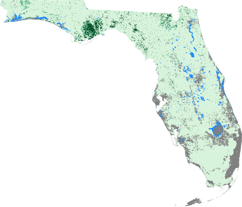
Lastly, we map the predicted results for the entire study area.

classified_image = embeddings.classify(classifier)

# Build the interactive legend dictionary dynamically from our mapping
legend_dict = {}
for code, desc in muc_level1_map.items():
    legend_label = f"{code}: {desc}"
    legend_dict[legend_label] = custom_palette[int(code)]

# Initialize the interactive map
Map = geemap.Map(center=[28.473813, -81.660044], zoom=9)

# Add classified image layer. We set min=0 and max=9 to perfectly align our 10-color palette
Map.addLayer(classified_image, {'min': 0, 'max': 9, 'palette': custom_palette}, 'Predicted Level 1 Land Cover')
Map.addLayer(local_fc, {'color': 'red'}, 'GLOBE Ground Truth Points')

# Add the built-in floating legend
Map.add_legend(title="Level 1 Land Cover", legend_dict=legend_dict)

# Display the Map
Map

from IPython.display import display, Image

# Define visualization parameters for the classified image
vis_params = {
    'min': 0,
    'max': 9,
    'palette': custom_palette,
    'region': region,
    'dimensions': 800, # Image width in pixels
    'format': 'png'
}

# Generate a direct URL to the static image from Earth Engine's servers
url = classified_image.getThumbURL(vis_params)

# Display the image in Colab
display(Image(url=url))