Modeling Mosquito Populations with AI and Earth Engine

We will train a simple AI model to predict mosquito populations using Google Earth Engine datasets and community science data.

Note: The mosquito observation data used in this lesson is from iNaturalist for 2020-01-01 to 2026-01-01. To keep the computational load light and avoid memory limits, we will train our model exclusively on data from 2024 and evaluate its predictions on 2025.

import pandas as pd
import geopandas as gpd
import ee
import geemap
from IPython.display import Image, display

Loading and Preparing the Data

First, we will load the data, convert the parquet file to a geodatabase using the latitude and longitude columns, and filter the points to Florida for a regional analysis. We will also print the number of points per year to understand our dataset.

# Load mosquito observations
url = 'https://github.com/geo-di-lab/emerge-geoai/raw/refs/heads/main/docs/data/mosquito_inaturalist_2020_2025.parquet'
df = pd.read_parquet(url)

# Convert parquet to a geodatabase (GeoDataFrame) using latitude and longitude
gdf = gpd.GeoDataFrame(
    df,
    geometry=gpd.points_from_xy(df.longitude, df.latitude),
    crs='EPSG:4326'
)

# Filter points to Florida for a regional analysis
fl_url = 'https://github.com/geo-di-lab/emerge-lessons/raw/refs/heads/main/docs/data/florida_boundary.geojson'
fl = gpd.read_file(fl_url)[['geometry']]
gdf_fl = gpd.sjoin(gdf, fl, predicate='within')

# Extract year and month from the observation date
date_col = pd.to_datetime(gdf_fl['observed_on'])
gdf_fl['year'] = date_col.dt.year
gdf_fl['month'] = date_col.dt.month

# Filter the dataset to include only June for the years 2024 and 2025
gdf_june = gdf_fl[
    (gdf_fl['month'] == 6) &
    (gdf_fl['year'].isin([2024, 2025]))
].copy()

# Print the number of points to verify the subset size
print("Number of June mosquito observations per year in Florida:")
print(gdf_june['year'].value_counts().sort_index())

# Keep only necessary columns for Earth Engine processing
gdf_clean = gdf_june[['year', 'geometry']].copy()

Number of June mosquito observations per year in Florida:
year
2024    59
2025    78
Name: count, dtype: int64

Preparing Environmental Inputs

We want to use proximity to water body, temperature, rainfall, NDVI, and NDWI as inputs. We will define a function to extract these environmental variables using Google Earth Engine.

To prevent memory limit errors during map generation, we will optimize our calculations by using a simplified bounding box for the thumbnail map layout. We will also compute water proximity using a set scale of 1000 meters.

# Authenticate and initialize Earth Engine
ee.Authenticate()
# Replace 'emerge-lessons' with your project ID if it is different
ee.Initialize(project='emerge-lessons')

# Convert Florida boundary and points to Earth Engine objects
fl_ee = geemap.geopandas_to_ee(fl).geometry()
mosquito_fc = geemap.geopandas_to_ee(gdf_clean)

# Create a simplified bounding box geometry for map rendering to prevent memory issues
fl_bounds = fl_ee.bounds()

# Function to extract environmental inputs for a given year
def get_environmental_inputs(year, region):
    start_date = f'{year}-06-01'
    end_date = f'{year}-06-30'

    # Temperature (MODIS Land Surface Temperature)
    temp = ee.ImageCollection('MODIS/061/MOD11A1') \
        .filterDate(start_date, end_date) \
        .select('LST_Day_1km') \
        .mean() \
        .rename('temperature')

    # Rainfall (CHIRPS Daily)
    rain = ee.ImageCollection('UCSB-CHG/CHIRPS/DAILY') \
        .filterDate(start_date, end_date) \
        .sum() \
        .rename('rainfall')

    # Vegetation and Water Indices (Sentinel-2)
    s2 = ee.ImageCollection('COPERNICUS/S2_SR_HARMONIZED') \
        .filterDate(start_date, end_date) \
        .filterBounds(region) \
        .median()

    ndvi = s2.normalizedDifference(['B8', 'B4']).rename('ndvi')
    ndwi = s2.normalizedDifference(['B3', 'B8']).rename('ndwi')

    # Proximity to Water Body (JRC Global Surface Water)
    water_mask = ee.Image("JRC/GSW1_4/GlobalSurfaceWater") \
        .select('occurrence') \
        .gt(0) \
        .unmask(0)

    # Find distance to the nearest water pixel using a set neighborhood of 256 pixels
    water_distance = water_mask.Not() \
        .fastDistanceTransform(256) \
        .multiply(1000) \
        .rename('water_distance')

    # Combine all inputs into a single image and clip to the study region
    combined_image = ee.Image([temp, rain, ndvi, ndwi, water_distance])
    return combined_image.clip(region)

Train/Validation Split and Model Training

Since these observations come from records submitted by people via iNaturalist, there are certainly mosquitoes that have not been observed. We will apply AI to fill in the gaps. We pair our known mosquito locations with randomly-generated background points, which represent areas without recorded observations.

To verify the accuracy and performance of our model, we will split our 2025 dataset into an 80% training set and a 20% validation set. We will use regression methods to map continuous mosquito prevalence.

# Define the environmental bands we will use as inputs
bands = ['temperature', 'rainfall', 'ndvi', 'ndwi', 'water_distance']

# Extract June environmental inputs for the training year (2024)
inputs_2024 = get_environmental_inputs(2024, fl_ee)

# Filter presence points for June 2024
presences_2024 = mosquito_fc.filter(ee.Filter.eq('year', 2024))

# Set prevalence to 1 for known mosquito locations
def set_presence(feature):
    return feature.set('prevalence', 1)
presences_2024 = presences_2024.map(set_presence)

# Generate random background points to balance the data
num_points = presences_2024.size()
absences_2024 = ee.FeatureCollection.randomPoints(region=fl_ee, points=num_points)

def set_absence(feature):
    return feature.set('prevalence', 0)
absences_2024 = absences_2024.map(set_absence)

# Combine presences and absences for June 2024
points_2024 = presences_2024.merge(absences_2024)

# Add a random column to split data into training and validation sets
points_with_random = points_2024.randomColumn('random')

# Split into 80% training and 20% validation datasets
training_points = points_with_random.filter(ee.Filter.lt('random', 0.80))
validation_points = points_with_random.filter(ee.Filter.gte('random', 0.80))

# Sample the environmental inputs for both datasets
training_data = inputs_2024.sampleRegions(
    collection=training_points,
    properties=['prevalence'],
    scale=1000,
    geometries=False
)

validation_data = inputs_2024.sampleRegions(
    collection=validation_points,
    properties=['prevalence'],
    scale=1000,
    geometries=False
)

# Train a Random Forest Regression model
rf_model = ee.Classifier.smileRandomForest(numberOfTrees=50) \
    .setOutputMode('REGRESSION') \
    .train(
        features=training_data,
        classProperty='prevalence',
        inputProperties=bands
    )

Model Evaluation

Now that our regression model is trained, we will test its performance on our validation data. Because the model outputs continuous prevalence scores rather than discrete classes, we evaluate accuracy using the Root Mean Squared Error (RMSE) and the Residual Sum of Squares to understand how closely our model fits the data.

# Classify the validation data to get predictions
validated = validation_data.classify(rf_model, 'predicted_prevalence')

# Calculate performance metrics
def compute_error(feature):
    diff = ee.Number(feature.get('prevalence')).subtract(ee.Number(feature.get('predicted_prevalence')))
    return feature.set('error_sq', diff.pow(2))

error_features = validated.map(compute_error)

# Calculate Mean Squared Error (MSE) and Root Mean Squared Error (RMSE)
mse = ee.Number(error_features.reduceColumns(ee.Reducer.mean(), ['error_sq']).get('mean'))
rmse = mse.sqrt()

print(f"Validation Root Mean Squared Error (RMSE) for June: {rmse.getInfo():.4f}")
print("An RMSE score closer to 0 reflects higher prediction performance.")

Validation Root Mean Squared Error (RMSE) for June: 0.3892
An RMSE score closer to 0 reflects higher prediction performance.

Creating Predicted Prevalence Maps for 2024 and 2025

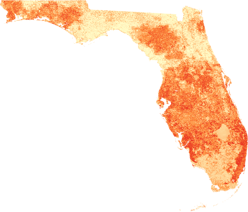
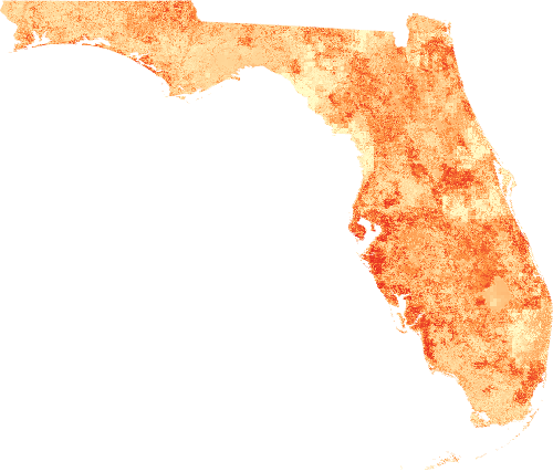
We can now use our trained model to map mosquito prevalence across the entire state for both 2024 and 2025. We will generate static maps for each year to visualize our predictions and inspect how changing climate variables alter potential habitats.

# Define visualization parameters for the map thumbnail
vis_params = {
    'min': 0,
    'max': 1,
    'palette': ['#ffffcc', '#fd8d3c', '#e31a1c'],
    'region': fl_bounds,
    'dimensions': 500
}

# Generate and display static map for June 2024
print("Predicted Mosquito Prevalence Map for June 2024...")
inputs_2024 = get_environmental_inputs(2024, fl_ee)
map_2024 = inputs_2024.classify(rf_model)
thumb_url_2024 = map_2024.getThumbURL(vis_params)
display(Image(url=thumb_url_2024))

# Generate and display static map for June 2025
print("Predicted Mosquito Prevalence Map for June 2025...")
inputs_2025 = get_environmental_inputs(2025, fl_ee)
map_2025 = inputs_2025.classify(rf_model)
thumb_url_2025 = map_2025.getThumbURL(vis_params)
display(Image(url=thumb_url_2025))